Information

This information is part of the Business Simulation Library (BSL).

From Business Process Modeling to Strategic Business Simulation

Business Process Modeling

Business process modeling (BPM) has become an ubiquitous activity in support of management decision making and business analytics. While there are different tools and notation for BPM, event-driven process chains (EPC) offer a very general and simple way of modeling business processes. Essentially, processes always start with an event that will lead to one or more activites (functions in EPC-terminology) which again will mount into one or more events, so that in general any activity must always be braced by two events.

Figure 1 shows an EPC for the idealized production process of ACME, a startup that produces intruder alarm systems specifically designed to meet private home owners’ needs. The diagram is valid for a single unit produced and shows events (red hexagons) and functions (green boxes) in typical notation.

Figure 1: Simple Production Process

While this "discrete-event" view of production is great for operational process improvement, it is not so well suited for for winning over investors by telling a compelling story about business development or for discussing policy-setting issues with regard to social systems and organizations. In these cases an aggregate strategic view is the better choice.

Aggregate View of Production

To go from the the familiar perspective of BPM to a more strategic one, we will look at what happens in a period. In a month there will be lots of events and actions. We can aggregate the actions and events separately: Individual actions will thus add up to a process that produces tangible results at a certain rate(e.g., assembled units per month). In the general case the rate may be a continuously varying quantity due to external and internal disruptions or policies. Events on the other hand can be collected as the countable results of processes, e.g., finished products can be collected in an inventory.

Figure 2 shows, how we can move from the event-driven process chain model to a strategic model using the Business Simulation Library. As in the EPC we will start out with its dynamic equivalent, a container—called stock. The very first stock is called a source in the library, which means that we assume infinite capacity indicating our model's boundary (i.e., in our example we do not care for the source of all material, that we need to assemble products).

Figure 2: Actions Add Up to Flows and Events to Stocks

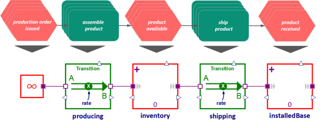The assembly of products in our example has been aggregated to a mere process of transition from the unlimited stock of raw materials to the inventory of finished goods. Shipping products in Figure 2 has also become a mere transition at some given rate, which moves our products to the stock installedBase representing continued use during the product's useful lifetime.

Stocks (with red color code inherited from events) and flows (with green color code inherited from actions) are atomic systems in the library. As we can see in Figure 2, stocks and flows are connected via acausal connectors (→ StockPort, → FlowPort). Each component reports basic information about what is going on inside using output connectors (white triangles; → RealOutput): A flow will report its current rate at any time during a simulation, whereas a stock will report the amount of entities that are inside at any time during a simulation. The numbers shown inside the stocks indicates the initial amount inside the respective stock.

Looking at the producing and shipping flows in Figure 2, we find, that they show a stylized pipeline (following System Dyamics conventions) with a stylized paddle wheel pump that is influenced by a variable called rate.

Figure 3: Setting the Rate

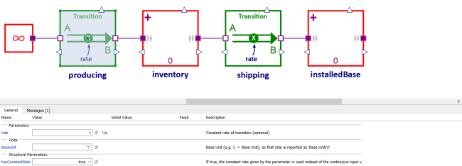Since there is no information input to the producing component, the rate of production in this simple case is a constant parameter. Figure 3 shows how—upon selecting the component—the rate can be set in the General tab in SystemModeler. Note, that there is also a structural parameter hasConstantRate that allows to instead of a parameter have an variable input for the rate.

Examples

This introductory example is continued in the package Examples:

SimpleProductionChain

SimpleProductionChainII

SimpleProductionChainIII